Integrating STARmap spatial transcriptomic and scRNA datasets using UINMF
April Kriebel and Joshua Welch
12/03/2021
Source:vignettes/articles/STARmap_dropviz_vig.Rmd
STARmap_dropviz_vig.RmdHere we demonstrate integrating a scRNA (Dropviz) dataset of the mouse frontal cortex and a spatial transcriptomics (STARmap) dataset of the same region. For this tutorial, we prepared the two datasets at a Dropbox folder
- The scRNA mouse dataset
Dropviz_starmap_vig.RDSis 28,366 genes by 71,639 cells. - The spatial transcriptomic STARmap dataset
STARmap_vig.RDSis 28 genes by 31,294 cells. - The annotation data of the Dropviz mouse data
Dropviz_general_annotations.RDS. - The 3D coordinate data of the STARmap dataset
STARmap_3D_Annotations.RDS
Step 1: Load the data
The datasets provided are presented in “dgCMatrix” class, which is a
common form of sparse matrix in R. We can then create a liger object
with a named list of the matrices. The unshared features should not be
subsetted out, or submitted separately. Rather, they should be included
in the matrix submitted for that dataset. This helps ensure proper
normalization. Different from other UINMF tutorials, we set the modality
of each dataset with argument modal, in this way, a slot
for spatial coordinates is preserved for the STARmap dataset.
Step 2: Preprocessing
2.1 Normalization
Liger simply normalizes the matrices by library size, without multiplying a scale factor or applying “log1p” transformation.
lig <- normalize(lig)2.2 Select variable genes
Given that the STARmap dataset has only 28 genes available and these
are also presented in the Dropviz dataset, we directly set all of them
as shared variable genes. Please use varFeatures<-()
method for accessing the shared variable genes. For the Dropviz dataset,
we further select variable genes from the unshared part of it. To enable
selection of unshared genes, users need to specify the name(s) of
dataset(s) where unshared genes should be chosen from to
useUnsharedDatasets.
lig <- selectGenes(lig, thresh = 0.3, useUnsharedDatasets = "dropviz", unsharedThresh = 0.3)## ℹ Selecting variable features for dataset "starmap"## ✔ ... 0 features selected out of 28 shared features.## ℹ Selecting variable features for dataset "dropviz"## ✔ ... 19 features selected out of 28 shared features.## ✔ ... 2775 features selected out of 28338 unshared features.## ✔ Finally 19 shared variable features are selected.
varFeatures(lig) <- rownames(dataset(lig, "starmap"))2.3 Scale not center
Then we scale the dataset. Three new matrices will be created under the hook, two containing the 28 shared variable genes for both datasets, and one for the unshared variable genes of the Dropviz data. Note that LIGER does not center the data before scaling because iNMF/UINMF methods require non-negative input.
lig <- scaleNotCenter(lig)Step 3: Joint Matrix Factorization
Unshared Integrative Non-negative Matrix Factorization (UINMF) can be
applied with runIntegration(..., method = "UINMF"). A
standalone function runUINMF() is also provided with more
detailed documentation and initialization setup. This step produces
factor gene loading matrices of the shared genes: \(W\) for shared information across datasets,
and \(V\) for dataset specific
information. Specific to UINMF method, additional factor gene loading
matrix of unshared features, \(U\) is
also produced. \(H\) matrices, the cell
factor loading matrices are produced for each dataset and can be
interpreted as low-rank representation of the cells.
In this tutorial, we set dataset specific lambda (regularization parameter) values to penalize the dataset specific effect differently.
Another noteworthy advantage of UINMF is that we are able to use a
larger number of factors than there are shared features. We captilize on
this by changing the default value of k to 40.
Step 4: Quantile Normalization and Joint Clustering
4.1 Quantile normalization
The default reference dataset for quantile normalization is the larger dataset, but users should select the higher quality dataset as the reference dataset, even if it is the smaller dataset. In this case, the Dropviz dataset is considered higher quality than the STARmap dataset, so we set the Dropviz dataset to be the reference dataset.
After this step, the low-rank cell factor loading matrices, \(H\), are aligned and ready for cluster definition.
lig <- quantileNorm(lig, reference = "dropviz")4.2 Leiden clustering
With the aligned cell factor loading information, we next apply Leiden community detection algorithm to identify cell clusters.
lig <- runCluster(lig)Step 5: Visualizations and Downstream processing
5.1 Dimensionality reduction
We create a UMAP with the quantile normalized cell factor loading.
lig <- runUMAP(lig)5.2 Plot UMAP
Next, we can visualize our factorized object by dataset to check the integration between datasets, and also the cluster labeling on the global population.
plotDatasetDimRed(lig)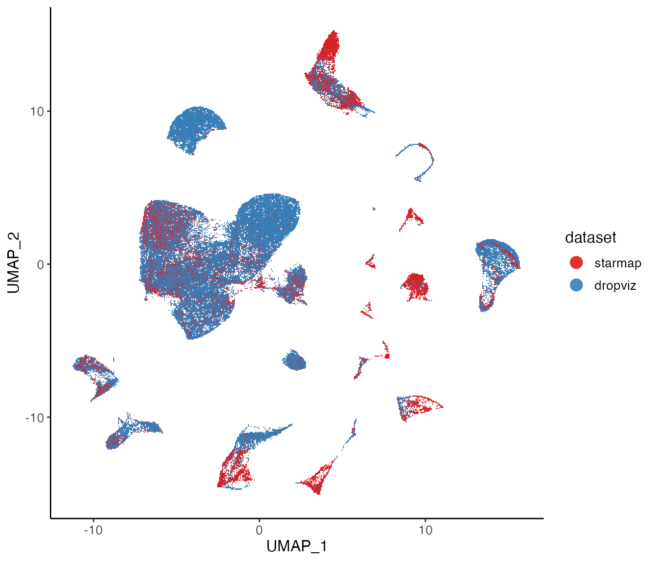
plotClusterDimRed(lig, legendNCol = 2)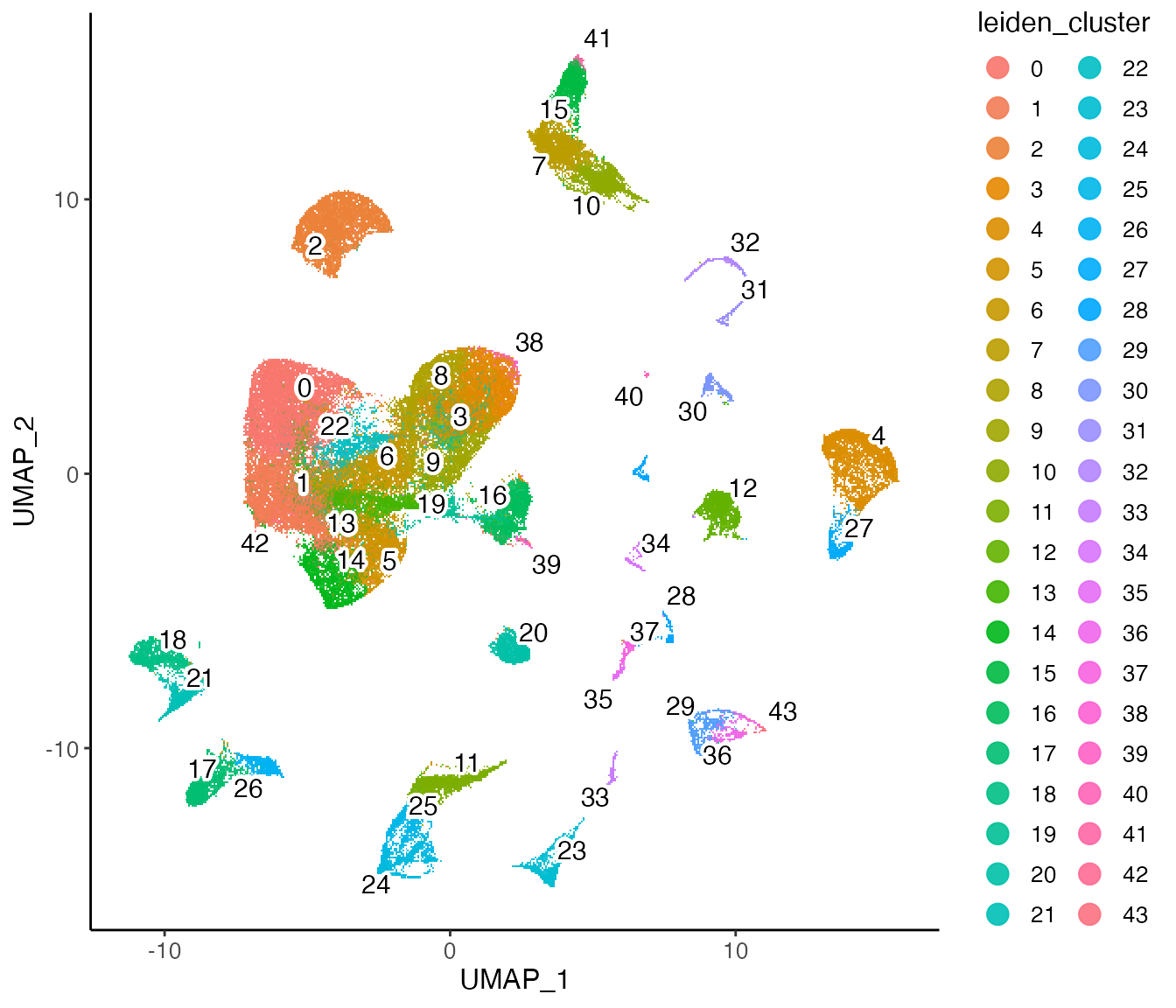
We can also use the Dropviz labels to help us annotate the clusters. Link to the downloading page of the labeling data is provided at top of this page.
mouse_annies <- readRDS("starmap_data/Dropviz_general_annotations.RDS")
dropviz_id <- paste0("dropviz_", names(mouse_annies))
cellMeta(lig, "dropviz_ann", cellIdx = dropviz_id) <- factor(mouse_annies)
plotClusterDimRed(lig, "dropviz_ann", legendNCol = 1)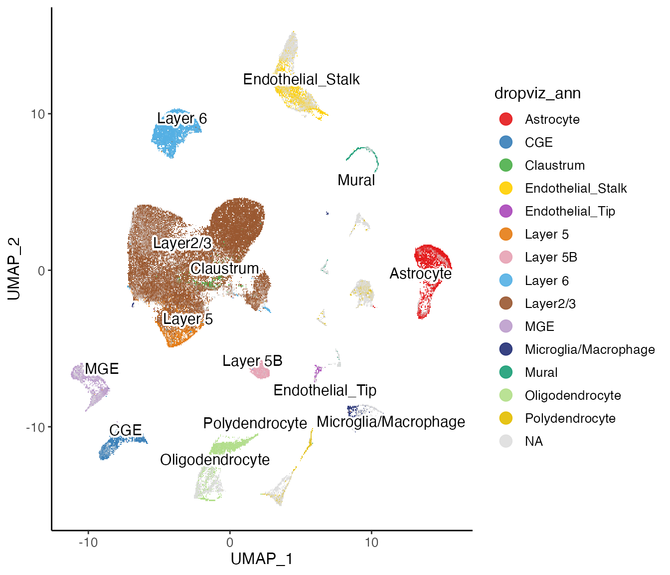
cellMeta()<- method has the feature for partial
insertion implemented and is great for adding dataset specific metadata
to a new variable. If you are unsure about the order between given
variable and the cells in the object, argument cellIdx can
be used for precise locating. Users might use different strategies when
creating the index depending on different situation.
Step 6: Visualization with spatial information
Here we demonstrate how to use the annotation labels derived from the above analysis within the context of 3D space. We provide the annotation labels for the sake of simplicity. The link to the download page is provided at the top of this page. These labels were generated using the high quality Dropviz annotations to re-annotate the STARmap cells after completing the above analysis. We have provided the exact annotations and colors used in the publication such that the interested user may captilize on the 3D dimensional sample space.
## Rows: 29,163
## Columns: 9
## $ Cell_Barcode       <chr> "starmap_11", "starmap_30", "starmap_51", "starmap_…
## $ Cluster            <fct> 15, 15, 15, 13, 15, 15, 13, 13, 15, 15, 1, 1, 15, 1…
## $ Cluster_Annotation <chr> "Layer 5A", "Layer 5A", "Layer 5A", "Layer 5A", "La…
## $ Coord1             <int> 12, 46, 81, 87, 92, 105, 117, 123, 128, 133, 170, 1…
## $ Coord2             <int> 937, 152, 76, 967, 948, 951, 284, 1004, 217, 319, 1…
## $ Coord3             <int> 8, 12, 7, 8, 8, 6, 7, 6, 6, 9, 6, 6, 7, 9, 6, 6, 6,…
## $ Cell_Type_Color    <chr> "plum", "plum", "plum", "plum", "plum", "plum", "pl…
## $ General_Class      <chr> "Neuron", "Neuron", "Neuron", "Neuron", "Neuron", "…
## $ Sub_Color          <chr> "#0066FF", "#0066FF", "#0066FF", "#0066FF", "#0066F…
6.1 Manage ligerSpatialDataset class (Optional)
Recall that we set the “modal” of the STARmap dataset to “spatial” when we created the liger object, here we can insert the coordinate information into the object.
coords <- as.matrix(starmap_annies[, c("Coord1", "Coord2", "Coord3")])
rownames(coords) <- starmap_annies$Cell_Barcode
coordinate(lig, "starmap") <- coords
LIGER does not yet have any analysis method that incorporate the
spatial coordinate information. Given that most of the spatial
transcriptomics technologies only support 2D spatial information, LIGER
only has 2D plotting (See plotSpatial2D()) method
implemented for the spatial coordinate at this point.
6.2 3D visualization
The STARmap technology we work with in this tutorial is special for 3D information. LIGER does not provide any function for the visualization of 3D coordinates, but here we provide a simple guide on it using package rgl.
The code chunk below shows how to create the 3D view of all cells.
library(rgl)

# Set the perspective parameters
rgl.viewpoint(theta = 25, phi = 5, zoom = 0.7)
# Generate scatter plot in 3D space
plot3d(x = starmap_annies$Coord1,
       y = starmap_annies$Coord2,
       z = starmap_annies$Coord3,
       xlab = "", ylab = "", zlab = "",
       col = starmap_annies$Cell_Type_Color,
       size = 2, axes= FALSE, labels = FALSE)
aspect3d(1.7, 1.4, 0.1)
first = c(0)
second = c(0)
# Set background color to black
bg3d("black", labels = FALSE)
axes3d(edges = "bbox",col = 'white', labels = FALSE, tick = FALSE)
As we can see above, cells of different types can be located at different depth (z-axis) and can interfere the observation of each other. We next show how to visualize with only neuronal cells.
# Subset annotation data to only Neurons
neuronal_cells <- starmap_annies[starmap_annies$General_Class == "Neuron",]
# Create 3D scatter plot with the subset
plot3d(x = neuronal_cells$Coord1,
       y = neuronal_cells$Coord2,
       z = neuronal_cells$Coord3,
       xlab = "", ylab = "", zlab = "",
       col = neuronal_cells$Sub_Color,
       size = 3, axes = FALSE, labels = FALSE)
aspect3d(1.7, 1.4, 0.1)
first = c(0)
second = c(0)
bg3d("black", labels = FALSE)
axes3d(edges = "bbox", col = 'white', labels = FALSE, tick = FALSE)