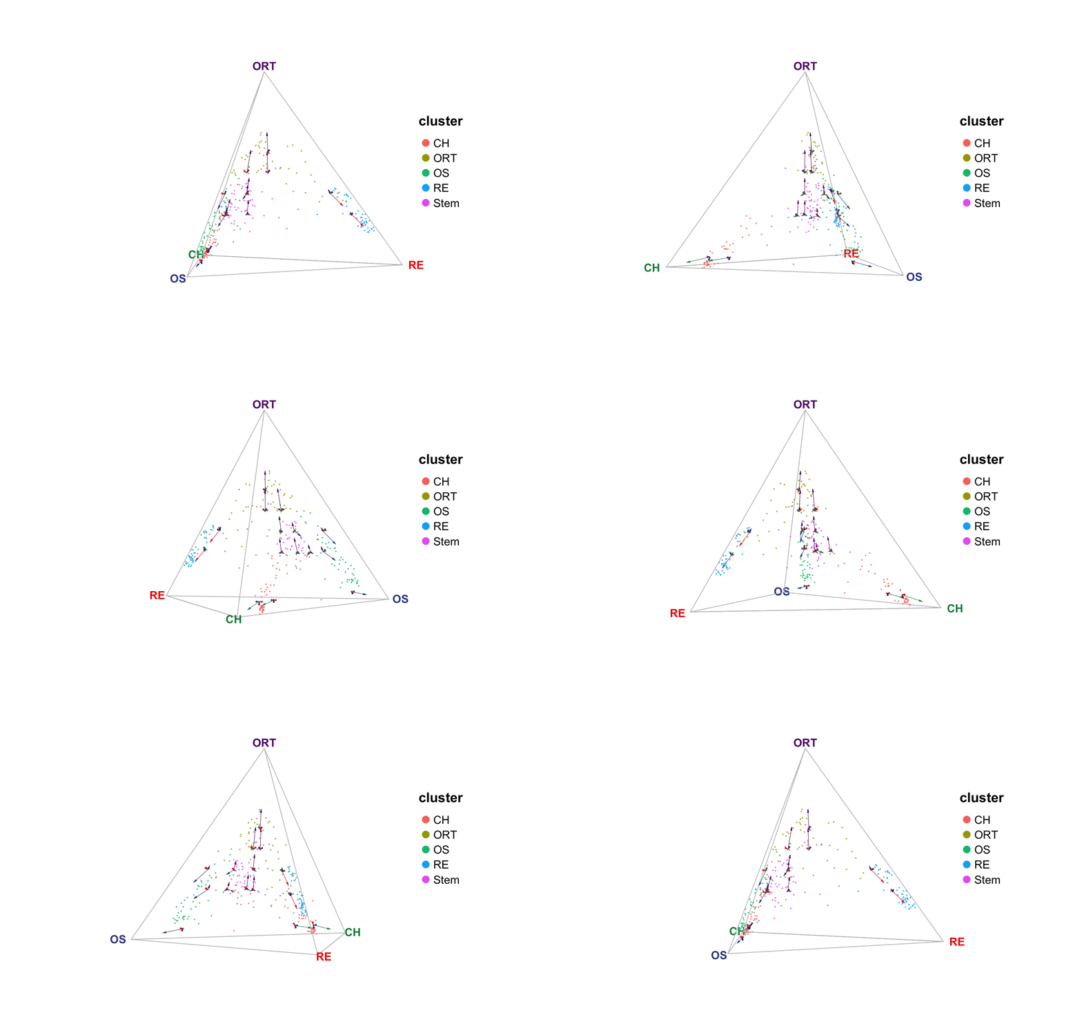
Simplex Visualization of Cell Fate Similarity in Single-Cell Data
Yichen Wang, Jialin Liu
04/23/2025
Source:vignettes/CytoSimplex.Rmd
CytoSimplex.RmdIntroduction
This package use simplex barycentric coordinate approach to assist
exploration in the similarity between single cells between selected cell
clusters. We denote a number (2-4) of selected clusters, or groups of
clusters, as vertices. We calculate the similarity between each single
cell and the average point of each vertex. By normalizing the similarity
between each single cell and all specified vertices to a unit sum, we
can derive a barycentric coordinate for each single cell. Visualization
method for binary (2-ended line), ternary (equilateral triangle) and
quaternary (tetrahedron) simplex are developed. The main plotting
functions are plotBinary(), plotTernary() and
plotQuaternary(), respectively. Please see full argument
documentation with ?plotBinary, ?plotTernary
and ?plotQuaternary. Here, we show some examples for
creating ternary and quaternary plots, which would be useful.
Example Data
In this vignette, we use data from Matsushita and Liu, Nat. Comm. 2023. The application of this method was originally used in this publicaiton as well. From the processed and annotated scRNA-seq data, we took the subset of 50 cells per major cell type from the raw count matrix and cell type annotation. These are embedded within this package.
library(CytoSimplex)
data("rnaRaw")
print(paste0("Class of `rnaRaw`: ", class(rnaRaw), ", dimension of `rnaRaw`: ", nrow(rnaRaw), " genes x ", ncol(rnaRaw), " cells"))
## [1] "Class of `rnaRaw`: dgCMatrix, dimension of `rnaRaw`: 20243 genes x 250 cells"## rnaCluster
## CH ORT OS RE Stem
## 50 50 50 50 50Select top features (optional but recommended)
Technically, any forms of feature-by-observation matrix is acceptable for the method we developed, and users are encouraged to explore the usability of our method with other types of data, even not biological. However, single-cell transcriptomics data, as provided, usually is of high dimensionality and contains technical and biological noise. With testing different approaches of reducing the dimensionality and noise, we recommend that users select a number of top differentially expressed genes (DEGs) for each cluster that a vertex represents.
We implemented a fast Wilcoxon rank-sum test method which can be
invoked with function selectTopFeatures(). Here, we will
choose the top DEGs for Osteoblast cells ("OS"), Reticular
cells ("RE") and Chondrocytes ("CH"), as also
shown in the previously mentioned publication. The number of top DEGs
for each cluster is set to 30 (nTop = 30), thus 90 unique
genes are expected to be returned. Alternatively, users can set
returnStats = TRUE to obtain a table of full Wilcoxon
rank-sum test statistics, including the result for all clusters instead
of selected vertices.
vertices <- c("OS", "RE", "CH")
geneSelect <- selectTopFeatures(rnaRaw, clusterVar = rnaCluster,
                                vertices = vertices, nTop = 30)
head(geneSelect)
## [1] "Nrk" "Eps8l2" "Mfi2" "Scin" "Fam101a" "Sox5"
stats <- selectTopFeatures(rnaRaw, clusterVar = rnaCluster,
                           vertices = vertices, nTop = 30, returnStats = TRUE)
head(stats)
## feature group avgExpr logFC statistic auc pval
## 1 Rp1 CH 0.0000000 0.0000000 5000.0 0.50000 NaN
## 2 Sox17 CH 0.0000000 0.0000000 5000.0 0.50000 NaN
## 3 Mrpl15 CH 8.4139185 5.7710321 6948.0 0.69480 7.500435e-08
## 4 Lypla1 CH 4.6278876 2.5075283 5894.0 0.58940 4.817036e-03
## 5 Gm37988 CH 0.2568508 0.2568508 5100.0 0.51000 4.659094e-02
## 6 Tcea1 CH 11.7897501 6.0049962 6559.5 0.65595 2.617836e-04
## padj pct_in pct_out
## 1 NaN 0 0.0
## 2 NaN 0 0.0
## 3 6.578978e-07 64 19.0
## 4 1.081562e-02 36 15.5
## 5 7.428025e-02 2 0.0
## 6 8.540867e-04 86 40.5Generating ternary plots
plotTernary() shows sample similarity in a ternary
simplex – equilateral triangle. The closer a dot, a cell, is to one
vertex, the more similar the cell is to the cell cluster(s) the vertex
represents. We recommend that users select the top marker genes for each
terminal and only use them as the features for calculating the
similarity.
vt.tern <- c("OS", "RE", "CH")
gene.tern <- selectTopFeatures(rnaRaw, clusterVar = rnaCluster, vertices = vt.tern)
plotTernary(rnaRaw, clusterVar = rnaCluster, vertices = vt.tern, features = gene.tern)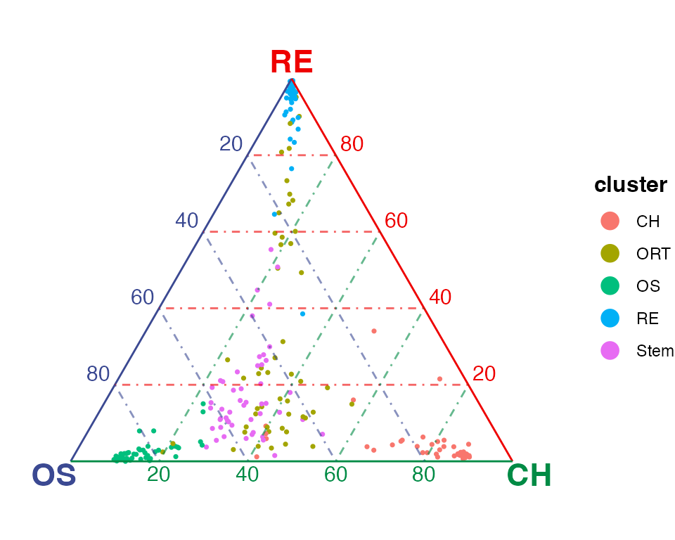
The static figure depends on
ggplot2, which is widely used for visualization in R. The binary simplex is plotted normally in ggplot 2D coordinates, while for the ternary simplex, the barycentric coordinate is drawn with 2D segments with cartesian coordinate, instead of implementing a ternary barycentric coordinate system. Users wishing to add customized alteration should pay attention to this.
Interactive ternary plot
The same figure above can be shown in an interactive panel, powered
by plotly. The interactive plot
allows users to zoom in and out, and hover over the dots to see the cell
names and the values of inferred similarity. To enable this feature,
users only need to add interactive = TRUE in the function
call.
plotTernary(rnaRaw, clusterVar = rnaCluster, vertices = vt.tern, features = gene.tern,
            interactive = TRUE)
For a rendered instance, please view our documentation website as the vignette is only allowed to demonstrate minimum content.
Adding velocity information to ternary plot
RNA velocity is a quantitative measurement of cellular transitions
from single-cell transcriptomics experiments and reveals transient
cellular dynamics among a heterogeneous cell population
(Qiao,
PNAS 2021). We implemented a velocity visualization strategy that
could be applied to ternary and quaternary simplex plot. The velocity
information input format must be an N x N graph (sparse matrix, where N
denotes number of cells). We have included a graph that matches with the
cells in the example dataset in this package. This graph is a subset of
the output from
Python
module veloVAE, as part of the processed data from the
publication mentioned at the start.
data("rnaVelo")
print(paste0("Class of `rnaVelo`: ", class(rnaVelo),
             ", dimension of `rnaVelo`: ", nrow(rnaVelo), " x ", ncol(rnaVelo)))
## [1] "Class of `rnaVelo`: dgCMatrix, dimension of `rnaVelo`: 250 x 250"We create a number of square grids in the 2D plain of the ternary simplex (or cube grids in 3D space of the quaternary simplex), and aggregate the cells fall into each grid with taking the mean of velocity towards each of the vertices. Finally, we draw an arrow from the grid center pointing to each vertex with the length representing the aggregated mean velocity.
Interactive view with velocity information is also supported. The aggregated potential value can also be shown when hovering above the arrows.
For a rendered instance of interactive visualization, please view our documentation website as the vignette is only allowed to demonstrate minimum content.
plotTernary(rnaRaw, clusterVar = rnaCluster, vertices = vt.tern,
            features = gene.tern, veloGraph = rnaVelo)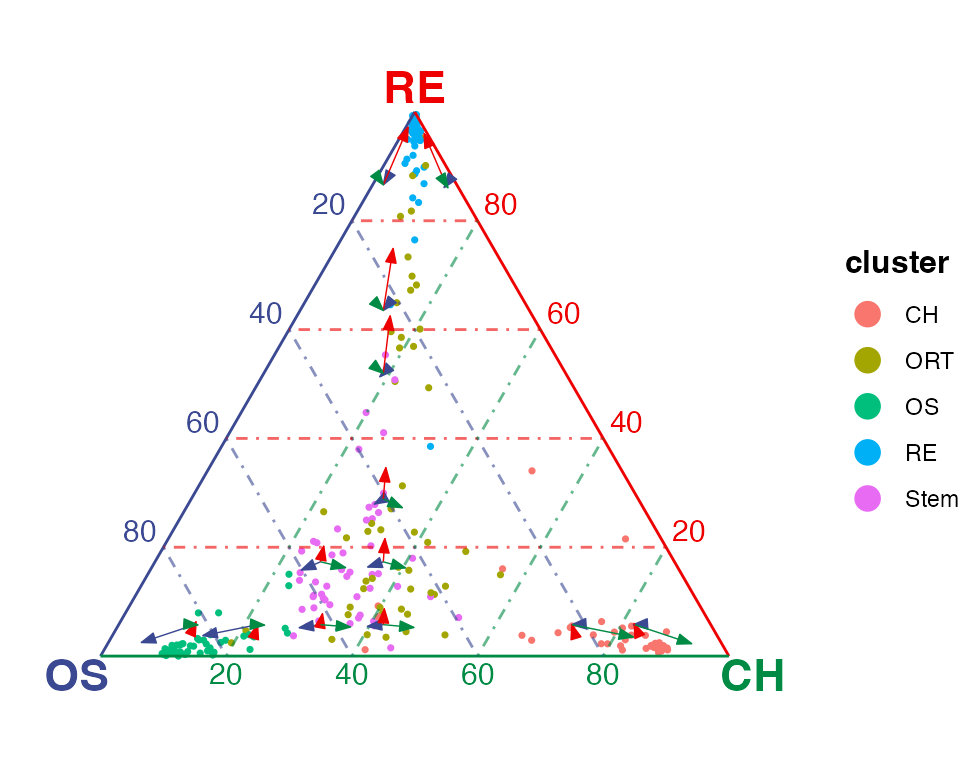
Exploration with each cluster
An argument splitCluster is supported for all three
plotting functions. By setting splitCluster = TRUE, A list
of plots will be returned, with one containing all cells, and each of
the other sub-plots containing only dots (cells) belonging to one
cluster in the annotation specified.
library(patchwork)
ternList <- plotTernary(rnaRaw, clusterVar = rnaCluster, vertices = vt.tern,
                        features = gene.tern,
                        byCluster = c("Stem", "RE", "ORT", "OS"))
print(names(ternList))
## [1] "Stem" "RE" "ORT" "OS"
(ternList$Stem + ternList$RE) / (ternList$ORT + ternList$OS)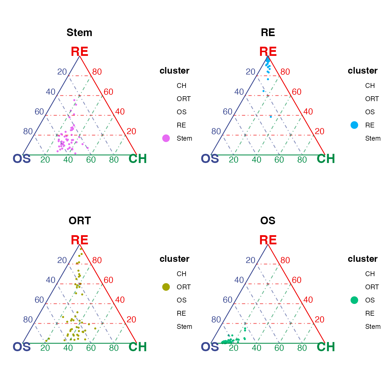
As can be seen in the subplots, osteoblast-chondrocyte transitional
(OCT) stem cells ("Stem") sit closer to osteoblast vertex
while do not tend to be extremely close to any vertex as observed in the
“OS” and “RE” clusters; reticular cells ("RE") and
osteoblast cells ("OS") are gathered towards their
corresponding vertices; osteoblast-reticular transitional cells
("ORT") distribute across the vertices for the two cell
types. These patterns match with the conclusion in the publication.
Similarly, the velocity layer can also be splitted.
veloSplit <- plotTernary(rnaRaw, clusterVar = rnaCluster, vertices = vt.tern,
                         features = gene.tern, veloGraph = rnaVelo,
                         byCluster = c("Stem", "RE", "ORT", "OS"))
(veloSplit$Stem + veloSplit$RE) / (veloSplit$ORT + veloSplit$OS)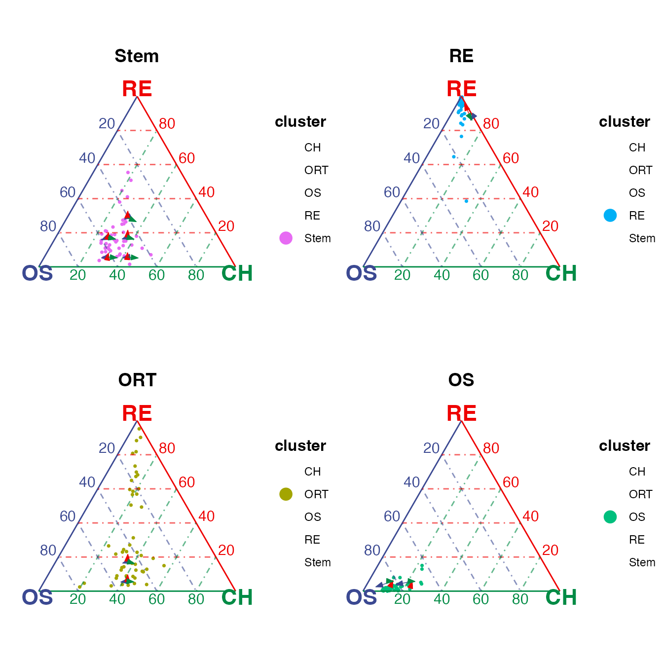
As shown in the subplots, the OCT stem cells has the transitional potential towards all three terminal cell types; reticular and osteablast cells are differentiating towards their corresponding cell types; while the ORT cells have the transition potential towards both osteoblast and reticular cell types.
Create quaternary simplex plot
For a quaternary simplex, we need one more cluster as a vertex. Here,
we add the cells annotated as osteoblast-reticular transition cells
("ORT") into the vertex list. We also add the velocity
information in this example, as it will not be shown by default. Note
that we provide interactive quaternary plot by default.
vt.quat <- c("OS", "RE", "CH", "ORT")
gene.quat <- selectTopFeatures(rnaRaw, clusterVar = rnaCluster, vertices = vt.quat)
plotQuaternary(rnaRaw, clusterVar = rnaCluster, vertices = vt.quat,
               features = gene.quat, veloGraph = rnaVelo, interactive = FALSE)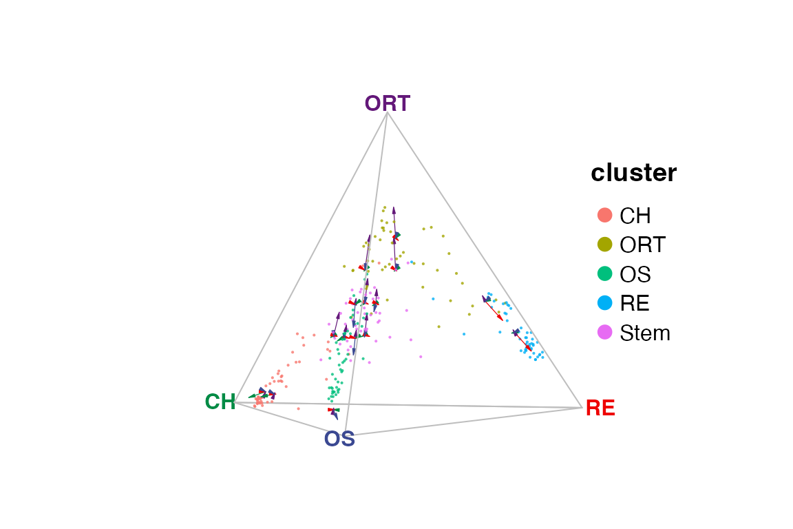
The default of
plotQuaternary()returns an interactive view. For a rendered instance of interactive visualization, please view our documentation website as the vignette is only allowed to demonstrate minimum content.
We have also implemented of GIF image generator that rotates the
tetrahedron rounding the z-axis. Note that package magick
is required for this feature.
(See
here for how to install magick in detail)
writeQuaternaryGIF(rnaRaw, clusterVar = rnaCluster, vertices = vt.quat,
                   features = gene.quat, veloGraph = rnaVelo,
                   width = 8, height = 5, res = 200)